![]()
![]()
![]()
![]()
![]()
![]()
|
|
||||||||||||
 |
||||||||||||
| chapter
four |
||||||||||||
|
Following the example set by the DIVA project (section 2.5) and further developed throughout chapter 2, it makes sense to exploit the similarities of instruments within MIVI. In this chapter, we describe how these commonalities are abstracted into hierarchical data structures and implemented in the MIVI code. We then continue to a lower level of abstraction and discuss how optimisations were made in the creation of the instruments graphics models, before discussing the implementation of a generic instrument class and both piano and flute subclasses. |
||||||||||||
|
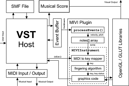
fig.4.1 - system structure and data flow
|
|
|||||||||||
| 4.1 hierarchical instrument definitions | ||||||||||||
|
In MIVI, we can capitalise on the similarities within instrument groups, as implicitly inherent in Yamaha XG and SONDIUS XG, when generating the instruments in 3D, by employing a hierarchical instrument definition. In our example of the string family, from section 2.2.3, many of its members can be defined using only a few parameters to dictate measurements and proportions, given a generic string instrument shape. This abstraction process is nothing new, and is similar to that conducted in the GLUT library of OpenGL (see Appendix B), where macros of lower level commands are used to create common primitives (cubes, sphere, etc.), given minimal parametised information. |
||||||||||||
|
As with the audible effects on sounds in physical modelling, the drivers for strings, themselves, remain almost visually unchanged from violin to viola to cello – for the bow, only the length changes, and for the hand (when plucking), no alteration is necessary. Thus to define a 3D bow and 3D hand for each string instrument, vertex-by-vertex, is exceedingly wasteful, and the introduction of a bow and hand sub-class, accessible to all members of a string instrument class makes for a more efficient approach. The hand sub-class will even lend itself to many other families and might benefit from an even greater – possibly global – scope. Other drivers prove equally as generic, as in the realm of percussion, where a drumstick class would come into play. |
||||||||||||
|
For instruments other than strings, the problem of abstracting similarities is yet more complicated. In the woodwind family, for example, clarinets, oboes and flutes have highly complex key layouts and configurations - each varying from one instrument to the next. It is no longer a case of just stretching a generic shape to attain the other members of the family. |
||||||||||||
|
abstracting instrument |
We must, instead, take our abstraction to a lower level and observe that although the layouts of each instrument vary, the styles and shapes of individual keys are repeated throughout the designs of the entire family, most appearing more than once in a single instrument. So, in the same way a GUI (graphical user interface) toolbar is an array of buttons, of varying styles (push button, on/off, icon, text, etc.), a MIVI wind instrument could be an array of instrument keys, with properties defining the various wind instrument key types (crook key, side key, trill key, closed key, etc.). Once the mechanism has been defined, it must simply be anchored to a separately defined instrument body. Unfortunately, the variety of wind instrument bodies makes factoring similarities at this level more difficult and, for now, it seems best to define them in the conventional vertex-by-vertex tradition. Besides efficiency, a further advantage of the abstraction approach will be the easy incorporation of degrees of freedom into the system. In the final animation of the instrument, it will be necessary for each key on the instrument to be independently moveable, as they would be on a real instrument. Thus, the computer is able to demonstrate how to play the instrument. The stack architecture of OpenGL, which enables such hierarchical modelling (see Appendix B), similarly allows us to implement causal key movements with minimal effort – where the position of one key affects the position of others, as is sometimes the case with wind instruments (eg. the D and D# keys on a flute). Similar approaches to those used in the woodwind section could be applied to brass. In this case, however, the fingering architecture (ie. the valves) is significantly simpler – sometimes nonexistent – and it is the pipe configuration that demands the attention. We shall not go into much detail here, but solutions could lie within the employment of interpolated curves, such as bezier or NURBS curves [3], which function like rubber hoses, with points along the curve strategically anchored at certain locations of the instrument, forcing familiar brass pipe shapes. Such a process, in effect, would mimic the actual method of brass instrument construction in the real world. Indeed, were the reader to also review texts on the manufacturing of most instruments [5][39], they would notice further adaptations of non-virtual construction techniques in the respective earlier discussions. |
|||||||||||
| 4.2 the 'MIVIInstrument' class | ||||||||||||
|
An instrument in the context of MIVI is far more than a simple 3D object. Aside from the aesthetical appearance, a MIVI instrument, just like a real instrument, must be able to respond to input dictated by music. Similarly, both have names, orchestral families and other properties implicitly associated with them. For these reasons, and those discussed in chapter 2, the introduction of a generic instrument class, MIVIInstrument (code ref. 07) will facilitate our design process. Extended instantiations of this class will form the various different instruments of our system, as visible from the front-end. A generic class contains operations and variables common to all its intended children; in this case the classes, miviPIANO (code ref. 08) and miviFLUTE (code ref. 09). The corresponding code is simply inherited from the parent and, thus, it is not necessary to write and rewrite it in each child class. |
||||||||||||
|
switching instruments |
Although
no more than one instrument will be used in MIVI at one time, we
wish to allow the user to change the active instrument at will,
without having to restart the program. Again, we do not want to
have to rewrite every feature The parent’s declaration (code ref. 07), although never instantiated and used directly in MIVI, acts as a specification for any given child class. If we initialise a pointer, *instrument, to an object of type MIVIInstrument, we can use this as a generic interface to any of its sub-types. All we have to do is direct the pointer to an object in memory of the appropriate sub-type, which encapsulates the desired instrument (code ref. 19). When a specific component of the MIVIInstrument pointer is called or queried, the directive is imparted to the active child sub-type, in our case miviPIANO or miviFLUTE. So, in our example, all that is now required is a single call to instrument->draw(). |
|||||||||||
|
initialising |
A common operation in this kind of object-orientated programming is one to initialise any instantiations of the object, setting components to default values, etc. In a normal class, this can be done in the constructor – in our case MIVIInstrument::MIVIInstrument(), which is called upon declaration. However, since the parent’s constructor will never be called, we create a dedicated initialisation procedure, init(), which can be executed from the active child’s constructor. Variables, range, octave and pitch, which govern the dynamic range of an instrument are assigned their default values here, following declaration in the class’ own declaration. Also, because this process is trivially short and simple, we take the liberty of defining the procedure’s body within the class’ declaration. These variables will allow us to marry the various keys and pitches of the instrument with a specified range in the global notes array – thus enabling MIDI-driven manipulation of the instrument. The first, range, simply tells us how many different pitches are in the range of the instrument. The second, octave, tells us the lowest octave the instrument is playable in. Finally, pitch aptly tells us the pitch in the aforementioned octave, from where the range begins. It is then assumed that the range is composed of pitches a semi-tone in separation, starting from the offset given by the latter two parameters and proceeding for range number of notes. |
|||||||||||
|
extending the |
Most instruments share these three characteristics, but for many, there will be extra properties unique to only that instrument – properties that will need to be available throughout the entire scope of the instrument’s class. For example, because the size of the piano’s body is dependent upon the size of the keyboard itself (which, in turn, varies depending on the number of keys), it is necessary to know the dimensions of the keyboard, before the body is drawn. Thus, at initialisation of our miviPIANO class, we deduce and set a global class variable keyboardWidth with the necessary information. Likewise, in the miviFLUTE class, it is necessary to have a variable indicating the current choice in fingering and, furthermore, to have flute-specific user-defined data types to support the construction and manipulation of the instrument. In each case, these variables and types must be set up in addition to the default trinity and are, thus, set up in the child’s own initialisation procedure. This time, however, we can move the code into the child’s constructor (code ref. 34 and 40, respectively), so that a new instrument can be created in a single – theoretically atomic – line of code. Note, we still retain the functionality of the parent’s procedure using an explicit call to MIVIInstrument::init(), re-queuing the call and its arguments on the parent. Inheritance and extension, not only applies to variables, but to operations too. Although every instrument must have some kind of draw() function, in order to produce the 3D model, each instrument may do this in a different fashion. Hence, although the draw() function is declared with null body in MIVIInstrument (to make it universally accessible to MIVI) and overridden in the child classes, extra abstraction may produce supplementary functions to aid drawing, such as drawKeyboard() or drawTube(), which are declared in only the child’s class declaration and called from the its draw() function. |
|||||||||||
|
4.2.1
integrating instruments into
VST |
||||||||||||
|
In VST, each plugin consists of a collection of ‘programs’, the concept of which is best illustrated by example. In the case of a Reverb (Reverberation) effect plugin, the programs would constitute effect presets, such as ‘Concert Hall’, ‘Canyon’, ‘White Plate’, etc. In MIVI, we could adapt this architectural feature and employ it to allow the switching of instruments, with our presets being ‘Piano’, ‘Flute’, Violin’, etc. In our implementation, we take this to a lower level and even specify the type of piano (categorised by the number of keys). In the typical VST plugin, this ‘program’ object has its own class, but in ours, we can absorb it as part of MIVIInstrument (code ref. 07), which we amend to be equivalent in the eyes of VST. Herein lies the raison d’etre for the name string (or character array). Upon initialisation, the host calls a plugin procedure getProgramName(), which must return the name of the active plugin. Using the second argument of the AudioEffectX constructor, identified and called as a parent plugin class in the plugin’s constructor, MIVI::MIVI() (code ref. 18), it cycles through n number of different programs – in our case, 5. Each is initialised, through setProgram() (code ref. 19), in order to extract its name, so that the host can present it to the user in a drop-down list, or other such form. Thus, by importing the name variable into our MIVIInstrument class and instantiating it inside the instrument’s constructor, we can emulate the ‘program’ functionality without the need for a dedicated ‘program’ class. Incidentally,
the inefficiency of this data collection method has |
||||||||||||
|
marrying instruments |
Along a similar line, the MIVIInstrument class also identifies any equivalent General MIDI voice number that the instrument might correspond to. The resulting variable, defaultGMvoice, is also set in the relevant constructor of the child instrument class. By doing this, instrument models could be selected using the simple 7-bit integer GM number. Thus, when the user changes the voice number of the track in the host, the ensuing Program Change MIDI message can be caught by processEvents() (discussed in section 5.1) and used to automatically switch to the appropriate instrument. However, the relatively confined variety of instruments, in our implementation, reduces the practicality of such a feature, at this early stage. |
|||||||||||
| 4.3 the 'miviPIANO' subclass | ||||||||||||
|
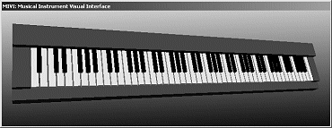
fig. 4.2 - the miviPIANO instrument model |
|
|||||||||||
|
The keyboard nature of the piano – and, hence, close conformity with the MIDI specification – makes it a good starting point for computerisation. The predictability and simplicity of the piano will allow us to test the system architecture. Furthermore, research in the field of music education [19][35] suggests that, after acclimatisation with the score, learning the piano is an advisable step before any other instrument. The end product is illustrated in Figure 4.2. As with the SONDIUS XG system, mentioned in the section 2.2.3, the appearance of the piano is a combination of driver and resonant body – keyboard and piano body, respectively. From a purely aesthetic point of view, these two components of the piano have little to do with one another and can be considered – and, thus, drawn – separately. The draw() function of the miviPIANO class (code ref. 35) illustrates this by having little more than a call to a function that draws the body and another call to one that draws the keys. The drawing technique behind each call, however, differs greatly. Of these, we will begin by explaining the former – the piano body. |
||||||||||||
|
4.3.1
the piano body |
||||||||||||
|
The piano case and keyboard are, of course, connected in terms of proximity and dimensions, namely width. Therefore, before drawing the body, we must know where and how big the keyboard is. To start, we simply assume all keyboards to have the same height and depth of key – variations of size are viewed proportional to the body, and thus can be accommodated by a scaling in that field. However, the width – defined by the number of keys – is variable and, unfortunately, due to the configuration of the piano’s keyboard, this is not simply a case of taking the width of a key and multiplying it by the number of keys. The existence and non-uniform distribution of black keys prevents this approach and, even though their dispersal pattern recurs in each octave (as defined by the pitch variable), because we can start at any offset within an octave (to accommodate all types of electronic keyboard), a simple algebraic equation for calculating the total keyboard width is not readily forthcoming. |
||||||||||||
|
making room |
Instead, using a similar algorithm to that employed to actually draw the keys, we simulate their creation and, instead of drawing the keys, increment a cumulative width variable in place of each white key. The calculation is performed by the function getKeyboardWidth() (code ref. 36), which is called in the miviPIANO constructor (code ref. 08), and returns a float representing the width. This is then stored in a class-scope variable, keyboardWidth, to enable access to it by any functions that require it. The algorithm employs two loops, one nested within the other. The first iterates through octaves, the second through the notes in the octave. The pattern of notes, on a piano, alternates between white and black except for every 3rd and 7th pair, where the black is absent. Hence, we simply guard the inclusion of black notes with a conditional statement to the same effect – if not the 3rd (j=2) or 7th (j=6) pair then draw a black note. Every time a note is drawn, we check that we have not met the limit on the number of notes (dictated by range) – terminating the loops if we have. Because the break statement only exits the closest nested for loop, we are forced to recheck the condition after exit, to enable us to exit the parent loop and subsequently, return the thread and result to the calling process. We take note of the octave offset, by pre-adding the missed notes (12 notes per octave × number of octaves) to the currentKey counter. In a similar way, we account for the pitch offset, but this also requires the first instance of the inner loop (notes in the octave) to be offset. This is done when the loop is first executed (when i=0 and j=0), by setting j to the appropriate next note. The structure of the loop demands that this be a white note, so the new j is determined from an array, nearestWhite, which maps the note of the pitch offset to the nearest white note. Ironically, the black keys, despite causing the initial dilemma, are not accounted for, as they merely overlap the whites’ real estate. Note also that this algorithm will produce incorrect (but non-fatal) results if the keyboard begins or ends with a black note. However, given the absence of such pianos in common use in the real world, this is not considered a problem. |
|||||||||||
|
the piano body |
In the piano’s case, excepting obscure forms of modern jazz, a pianist only manipulates the driver and, thus, the body will largely be a static object. We can take advantage of this fact by knowing a little about how OpenGL communicates with the graphics hardware, and using OpenGL display lists (explained in Appendix B). The body list is ‘compiled’ in the function initBody() (code ref. 37), which, ideally, we only want to call once per instrument outing. So, at first, it would appear sensible to call the function during the instrument’s constructor. However, it is possible that the draw() function is called before this procedure, through an eager idle() call from the host. Thus, before calling the procedure to draw the list’s graphics, in draw() (code ref. 35), we check that the list is non-zero. If we find that it is zero, then we call initBody() to rectify the situation. This also means that we can post updates for re-compilation of the body by simply setting body to 0 explicitly. So, when the parameters affecting keyboardWidth, which, in turn, affect the body, are changed, the constructor can force the body list to recompile accordingly. Further evidence of OpenGL’s lack of support for sub-windows emerges when we see that any compiled display lists are lost when our OpenGL window is destroyed. Because our window can be closed without terminating the plugin, our MIVIInstrument object can persist without a body list. Thus, when we re-open the window, the instrument body is drawn from an empty list – it does not exist. We must, therefore, post an update for recompilation, which we do through the calling of the MIVIInstrument::reinit() (code ref. 26), and is defined in the MIVIInstrument constructor (code ref. 07). As before, this function merely sets the variable body to 0. On a positive note; in order to change the style of the piano (from upright to grand) for example, we could simply place a switch statement in the initBody() procedure, which, conditional on the active style, will compile the appropriate piano body-style code accordingly. So, just as the *instrument pointer provides a generic interface to the MIVIInstrument type, body also represents a single point of contact to the piano body’s 3D object. |
|||||||||||
|
drawing the case |
In the move from runtime interpretation to compilation, no change in syntax or grammar is required, and we can specify the 3D shapes and attributes in the traditional OpenGL way. To create our body (code ref. 37), we simply position and stretch four cubes, which are created using the GLUT shape macro glutSolidCube(). Each time, the modelling matrix is stretched using glScalef() beforehand, so the function returns an appropriately extruded quadrilateral – a cuboid, as opposed to a cube. The final two, forming the ribs at each of the keyboard, are identical in all respects save location. Thus, we place them in a loop that calls the same functions, but varies the translation parameters between the two iterations. Once we have specified the body graphics, we call glEndList(), which will convert our high-level language into bits and bytes, ready to be sent to the hardware with glCallList(). |
|||||||||||
|
4.3.2
the keyboard |
||||||||||||
|
The situation is different when dynamism is required, as in most instrument drivers. For instance, in piano keys, we require freedom of movement for each key and the ability to change their attributes, such as material (for highlighting purposes). Therefore, it is unfortunately necessary to execute the varying commands at the higher interpreted level, as is done in drawKeyboard() (code ref. 38). |
||||||||||||
|
Unlike some – notably monophonic – instruments (as we shall see, in the case of the flute, later), the piano boasts the simplest mapping of MIDI pitch to key possible – one to one (1:1), a bijective function. Put simply, within a defined range, each MIDI pitch corresponds to exactly one key on the piano keyboard and vice versa – each key on the keyboard corresponds to exactly one MIDI pitch. Interestingly this is not true for the score, which is many to one, a non-injective function, since one pitch can normally be expressed in at least two ways using accidentals – an Eb is equivalent to a D#, and thus the same key. Thus, as we did in the getKeyboardWidth()function (see section 4.3.1), we can iterate through octaves and octave notes, simultaneously drawing the keys and incrementing the currentKey counter. At each point where a key is created, the counter will unite the 3D object with a note object in the notes array by using the current value of currentKey as the array’s subscript. Again, as in getKeyboardWidth(), we align the two scales at the outset, so as to correctly line up the instrument’s dynamic range with the right domain of the array. Now, displaying the condition of the note is a simple matter (code ref. 39). Before we draw the key, we inspect the corresponding status in the notes[currentKey] variable. Outside of the tutor system (discussed in section 5.2), it is simply a matter of checking to see if the note’s velocity is non-zero. Depending on the result and the display preferences set by the user, the key can be depressed (by translating it) or highlighted (by changing the material) or both. Otherwise, if TUTOR_MODE is set to true, we need to adorn the keys with performance directives and tutor instructions. Hence, prior to creation of the 3D keys, which are, in essence, stretched cubes, we use the rules (discussed later in section 5.2.3) to assign the appropriate material for each key (as defined at the beginning of the procedure) with glMaterialf() and properly displace them with glTranslatef(). |
||||||||||||
|
utilising the OpenGL stack architecture |
Notice, however, that after sinking a white key, we do not have to rise back up before creating the next. This is due to our use of the OpenGL stack (as discussed in Appendix B). Instead, all we have to do is pop the stack, thus reverting to the same position we were in before the key was created – where we last pushed the stack. To move to the base of the next key we simply translate the ‘cursor’ along, horizontally. Further inspection of the code shows that the creation of a black keys, through the use of the stack, results in no net movement of the cursor, as reflected in the code for getKeyboardWidth(), previously discussed. The stack will make itself even more useful when we it come to implement the key mechanism of the flute. |
|||||||||||
| 4.4 the 'miviFLUTE' subclass | ||||||||||||
|
fig. 4.3 - the miviFLUTE instrument model |
|
|||||||||||
|
In many respects, the flute lies at the opposite end of the musical instrument spectrum to the piano. It is driven by breath, can only play a single note at once (monophonic15), small, portable, often metal (though a ’woodwind’ instrument) and produces a completely different timbre of sound. Thus, a successful implementation of a miviFLUTE class, as a progression from our miviPIANO class, should demonstrate the universal applicability of the MIVI concept in a wide range of instruments and music education in general. In this project, we implement a Boehm flute [5], as pictured in figure 4.3, without the common modern extension of Briccialdi’s Bb thumb lever or the Dorus Key. |
||||||||||||
|
common traits |
However, let us start with what we already know. Like the piano, the flute’s defaultGMvoice and name are set in the constructor (code ref. 40) and the default initialisation code of MIVIInstrument is called. Similarly, the flute’s physical structure is segregated into static and dynamic parts – the flute body and key mechanism – and, like the piano’s, the flute body’s 3D graphics are pre-compiled in initBody() (code ref. 42) using OpenGL display lists. It, therefore, follows that the draw() function (code ref. 41) also shares a similar dynamic nature with that in miviPIANO. Overall, these front-end aspects of the miviFLUTE class allow it to be considered, as seen by the rest of the MIVI plugin, equivalent to miviPIANO and MIVIInstrument, permitting the latter’s use as a generic interface to the instrument. Inspecting and comparing the two instrument’s class declarations, however, we see that the principal difference lies in the private scope – once given a generic task, such as ‘draw the instrument’, each sub-class uses its own unique methods and architectures to execute it. |
|||||||||||
|
4.4.1
the flute body |
||||||||||||
|
Superficially, the shapes of bodies differ. Although there is little remarkable about this, in itself, the initBody() function (code ref. 42) does introduce the use of the functions drawTube() and drawRib(). These are the flute’s own local OpenGL shape macros. As is visible in the source code, the tube shape – a cylinder with ‘bevelled’ ends – not only represents the main body of the flute, but when appropriately scaled, the rods and even keys, as well. It is therefore useful to have this code separate and simply call it when needed, exactly as we do with the GLUT function glutSolidCube() in the miviPIANO class. The function drawTube() (code ref. 49) simply draws three strips of quadrilaterals; one for the mid section and one for each of the ‘bevelled’ ends. In the latter case, one edge of the strip is anchored at a single point in space, resulting in a cone-shaped appearance, giving the cylinder a crude, but effective, rounded or bevelled cap. The function drawRib() (code ref. 50) exploits drawTube() by simply scaling the result in one dimension to produce a more disc-like form. The initBody() procedure simply executes one large cylinder with drawTube(), ribbed at 3 points with drawRib(), to denote the common separable segments of a flute. |
||||||||||||
|
4.4.2
the key mechanism |
||||||||||||
|
From just initial inspection and impression, a large difference between the piano and flute instantly makes itself known – the fingering, or key, mechanism. Far from being a regular pattern of ivory white and ebony black keys, the flute seems a chaotic muddle of metal rods, tubes, axles and buttons. Far from chaos theory, the mechanics of the flute are almost literally the art of science16, but cannot nonetheless be encapsulated in a simple recursive algorithm, which relies on repetition and regularity. |
||||||||||||
|
Thus, resulting from this elaborate mechanism, another big difference from the piano is how the flute is played. Instead of a simple 1:1 function of note to key, as in the last section, the flute’s key mechanism boasts a far more complex mapping, where, more often than not, several keys must be pressed to produce even one solitary pitch. Additionally, due to the finite and limited number of available keys, any one key can reappear as a constituent of any number of other pitch fingerings. Furthermore, the flute is such that there is sometimes more than one way to finger a single note. Yet another problem appears when we take a closer look at the flute’s construction. Each key can be of a variety of shapes and is connected to an axle. An axle can simultaneously be home to other such varying keys and, itself, can form but one of many axles in a rod. The rods serve as a shaft, which allow the axles to rotate. The keys, axles and rods are connected so that, when a key is pressed, not only will the hole (under the key) in the flute’s main air tube, be closed, but so will any hole under any key connected at any point along the entire axle. Thus, technically, it is not only notes that map to keys, but other keys too. It should already be obvious, to the reader, that simply aligning a variable like currentKey, as before, will not be enough to properly represent and identify the notes on the instrument by itself. Instead, we need to devise of a method of encapsulating the instrument in data, then constructing an algorithm that can, given the data, construct our 3D model. For this we take a largely object-oriented top-down approach and use the structure of the instrument in the real world to base our simulated model on. This suggests the definition of different data types for keys, axles and rods. However, since the axles appear inside the rods, they will not be visible in the 3D model, and we take the liberty of omitting their explicit implementation. Instead, we will emulate the causal effects of one key press over another in the definition of the keys themselves.
|
||||||||||||
|
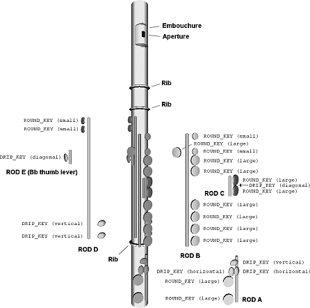
fig. 4.4 – structure of our flute model |
|
|||||||||||
|
implementing |
First, however, we must provide a foundation for the keys – the rods. In appearance, they are no more than long thin cylinders placed at certain angles and heights around the tube, and this is exactly how we can define them. The array rods (code ref. 43) is of type fluteRod. Each fluteRod (code ref. 12) comprises of the components vOffset, denoting the rod’s position along the flute body from the base, length, aptly denoting the length of the rod, and pOffset, denoting the (polar) angle of the rod around the main body. In the array, we give the specifications of the five rods, characteristic of a typical Boehm flute. Then later (code ref. 47), we iterate through each, performing the appropriate translation, scaling and rotation (respectively) before drawTube() is used to actually create the rod. |
|||||||||||
|
implementing |
Like the flute’s rods, we give its keys their own data type, aptly named fluteKey. Similarly, we use this type to construct an array, keys (code ref. 47), encapsulating all the keys in the flute model. To marry the various keys with their respective rods, we add an extra dimension to the keys array, where the subscript identifies the rod. The variety and functionality of keys make the key type far more complicated than that of the rod, which we can see by looking at the declaration of the fluteKey type (code ref. 13). This time, instead of a distance along the flute’s body, we define vOffset as the key’s distance along its rod. However, we use this component in much the same way – as a parameter to a translation function. Next, we identify the shape of the key, in the type component, given a small selection of key shapes – defined in the enumerated type keyType (code ref. 11). Later, this is used in a conditional statement to select appropriate code to draw the desired shape. The direction component simply tells us whether the key points clockwise or anti-clockwise around the tube, using an enumerated type (code ref. 10). Then, because the different key types and shapes have different properties, the next three float components are reserved to handle these extra data. For example, a ROUND_KEY can vary in size, whereas a DRIP_KEY (such as a trill key) can change both length and orientation. These parameters, like vOffset, are brought to bear when the keys are drawn and are, similarly, passed to functions like glScalef(), glRotatef() and glTranslatef(). However, their context – and thus their use – is determined by way of the previous type component. The final two attributes relate to how the instrument is fingered, and thus require knowledge of our fingering implementation. The structure, as it relates to the instrument, is illustrated in figure 4.4. |
|||||||||||
|
implementing |
Thinking about how a flautist would approach a note on the page, we see that we need a one to many (non-injective) relation, where one note, on the stave, causes the player to depress a certain combination of keys. Thus, we need an array where each member represents a configuration of key presses and whose range is a subset of the notes array’s total domain, equal to the range variable. Within this interval, which should correspond to the entire dynamic range of the flute, the relation between these two dimensions is, itself, 1:1 – one fingering combination to each note. Thus, when the time comes, the lookup can be performed using a variable representing the note, similar to the original currentKey counter, as the subscript. The structure of each fingering configuration, encoded in the fingerings array (code ref. 45), is simply a collection of 1’s and 0’s, where each ‘bit’ tells MIVI if the key (associated with the bit’s offset) is pressed or released. When it comes to drawing the keys, the procedure will iterate through the keys array, making it sensible to define the relation between key and offset as part of the fluteKey type. This is achieved using the finger component, which enables the mapping of flute key to fingering configuration offset. |
|||||||||||
|
monopolising |
Because of the flute’s monophonic nature, this currentKey equivalent for the flute will only represent one note throughout the drawKeyMechanism() procedure. However, the notes array, supplied by MIVI, still holds the information for all pitches – instead of explicitly telling miviFLUTE which note is being played, it broadcasts the status of all notes. |
|||||||||||
|
MIVI’s notes array is by definition polyphonic, to allow for the handling of pianos and other such instruments. Indeed, most MIDI output devices will accept and play a polyphonic input, even through a flute voice. In our VST host, there is nothing to stop chords being transmitted to the MIVI flute. Thus, before embarking on any graphics operations or fingering decisions, we must cycle through the array and find which one note is on. Since this is likely to be a popular operation amongst monophonic MIVI instruments, we export this simple monopolising algorithm to the global MIVI scope, as the function getMonoPoly() (code ref. 32). Note, however, that the loop cycles from the top end of the array down. The array will return the first note, so, in the event that a multiphonic signal, such as piano music, is passed to the function, it has an outside chance of extracting the normally higher melody line (or ostinato) from the right hand’s notes. Similarly, the algorithm could be amended to iterate in the other direction, to siphon out any bass line, more useful in bass instruments like the bass guitar and double bass. Such filtering techniques grow in complexity very quickly and present an interesting area of study, auto-arrangement [12] – where various unassigned lines of music are automatically distributed about the instruments of an ensemble (often the orchestra), based on pitch, complexity, required skill and other characteristics. |
||||||||||||
|
optimal fingering |
The process becomes more complex when we are forced to decide between multiple fingerings – our 1:1 mapping of note to fingering becomes 1 to many again. This time, though, we deterministically choose a result in the domain. We store these alternative configurations, as an extra dimension of the fingerings array. However, alternate fingerings do not exist for all notes, so we must somehow mark those that do. Extending the information stored about each configuration to additionally flag the existence of an alternative configuration, achieves this. Now, not only need we only make a decision when this flag is set, but if more than two fingerings were to be available, the same test can be performed on the alternative configuration to check if yet more are available. This, of course, can continue recursively, in much the same fashion as a linked-list. At this point, we are ready to implement code (code ref. 46) to decide which configuration is best, given an alternative. Because Boehm’s book states the existence of, at most, two fingerings per note, we will forego the implementation of a recursive decision maker, and simply compare the two directly. Fingering algorithms, as discussed in the section 2.3.2, are already a subject of advanced study and debate, so little would be gained by attempting to produce an algorithm anything more than practical for our purposes. Hence, when a change of note is detected, and thus a change of fingering is warranted, we compare both the fingerings with the previously chosen fingering, penalising them for change in individual finger position they require. After the loop, which iteratively does this for each finger, ends, the decision variable favourDefault will be used to set the cheapest new fingering. The choice is then assigned to the currentFingering object, which is of type fingering (code ref. 14). A fingering object has two components; bank, which identifies which dimension of the fingerings array the fingering in question belongs to, and note, which is used to index that dimension of the fingerings array and simply represents the pitch (as returned by getMonoPoly()). With this, we revert to a 1:1 mapping of note to fingering |
|||||||||||
|
drawing the keys |
This gives us enough information to proceed with the creation of the 3D model. To this end, we iterate, again with two hierarchical loops, through each rod (code ref. 47) and each rod’s keys (code ref. 48), respectively. Though the rods are simply a product of their parameters, the keys, which must present meaningful information to the user, are more involved. We know the current note and, thus, the current fingering configuration. So, at the creation of each key, we can lookup in the fingerings array the offset dictated by the current key’s finger component (2nd subscript), of the bank we chose to be the optimal (1st subscript), and see if the key should be depressed or not, given the current note (3rd subscript). Before doing so, however, we check to see if the key is fingerable in some way, by verifying that the finger component is non-zero. |
|||||||||||
|
axle emulation - dependent keys |
As mentioned, when a key on one axle is pressed, it closes other keys on the same axle simultaneously. Thus, we consider these keys as children of other keys, who must obey their parents. The mysterious three parent components of the fluteKey type thus follow a similar principle to the finger component. When their parent keys are denoted depressed in the fingering configuration, they must be depressed too. We use a simple iterative loop to repeat checks, similar to the finger component, for each of the three parents. |
|||||||||||
|
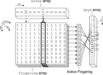
The mapping of note to key, as implemented in our system, is illustrated in figure 4.5. In it, one (monophonic) pitch from the notes array, monopolised by getMonoPoly(), denotes the active fingering of the fingering array. Then an optimal fingering algorithm denotes the active bank of the fingering array. These two values are stored in the currentFingering object’s fingering and bank component respectively. In the diagram, ‘Active Fingering’ represents the fingering identified, and each member correlates with a key on the flute, encoded as a fluteKey in the keys array. Finally, our axle-emulation ensures that the non-fingered keys are also depressed appropriately. Any depressed keys are emphasised in the diagram. |
||||||||||||
|
fig.4.5 - mapping of note to key |
|
|||||||||||
|
A problem, however, arises when the user is learning how to finger their own instrument, and when several keys go down at once – they must arbitrarily decide which should be pressed. No computer-generated fingers, as yet (see section 7.1), exist to relate this information. So, we resort to our second display mode – highlighting. All we must do is present the fingered keys and dependent keys in different colours. For this, we choose our default red for the first, and a less saturated red – pink – for the second. Indeed, it is not necessary to highlight the latter keys at all, so we make this extended feature explicitly toggleable on the interface (see section 5.3). Depending on the display mode set by the user, the results of these checks and lookups will have different influences. For example, regardless of whether the key is active due to fingering or due to dependency, we want to depress it when in DEPRESS_MODE. However, in the highlight modes, the key’s material will change in each case. Thus, it is wise to hold off any graphics operations until the results are known. This way, we avoid having to repeat such operational code in each conditional branch – both the finger and parent checks. Instead, we flag the results, in the two-bit Boolean array noteOn, so that, later, we can use simple bit-wise comparators to set the appropriate mode later. The remaining code simply uses the parameters of the keys array to draw the flute’s key, where the ROUND_KEY uses our proprietary tube macro and the DRIP_KEY, GLUT’s sphere macro. |
||||||||||||
|
exploiting the OpenGL |
Throughout the code are littered the commands glPushMatrix() and glPopMatrix(), which, as we discovered in our discussion of the piano code, manipulate the stack, storing the OpenGL ‘cursor’ for later retrieval. In the flute model, this tool is used to a far greater extent. Whereas in the previous case, most of stack operations could be easily implemented manually (by simple return glTranslatef() functions), the variety of flute rod positions and rotations coupled with those of the individual flute keys (which also add scalings) would, this time, make a similar approach far more difficult and costly. Instead, we push to the stack when we start each rod, so that when we have finished drawing it, we need only pop it to continue with next in the same fashion. Likewise, we do exactly the same thing with the keys on the rods themselves; after each key, a single glPopMatrix() command returns us to the base of the rod. |
|||||||||||

![]()
All content,
including code and media, (c) Copyright 2002 Chris Nash.